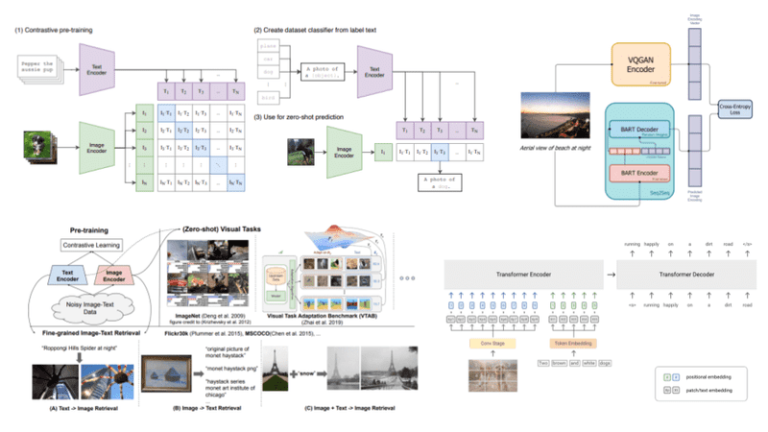
Multimodal learning refers to the process of learning representations from different types of modalities using the same model. Different modalities are characterized by different statistical properties. In the context of machine learning, input modalities include images, text, audio, etc. In this article, we will discuss only images and text as inputs and see how we can build Vision-Language (VL) models.
Vision-language tasks
Vision-language models have gained a lot of popularity in recent years due to the number of potential applications. We can roughly categorize them into 3 different areas. Let’s explore them along with their subcategories.
Generation tasks
Visual Question Answering (VQA) refers to the process of providing an answer to a question given a visual input (image or video).
Visual Captioning (VC) generates descriptions for a given visual input.
Visual Commonsense Reasoning (VCR) infers common-sense information and cognitive understanding given a visual input.
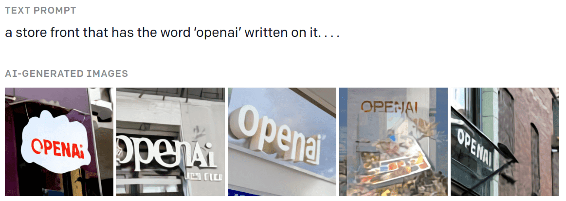
Visual Generation (VG) generates visual output from a textual input, as shown in the image.
Source: OpenAI’s blog
Classification tasks
Multimodal Affective Computing (MAC) interprets visual affective activity from visual and textual input. In a way, it can be seen as multimodal sentiment analysis.
Natural Language for Visual Reasoning (NLVR) determines if a statement regarding a visual input is correct or not.
Retrieval tasks
Visual Retrieval (VR) retrieves images based only on a textual description.
Vision-Language Navigation (VLN) is the task of an agent navigating through a space based on textual instructions.
Multimodal Machine Translation (MMT) involves translating a description from one language to another with additional visual information.
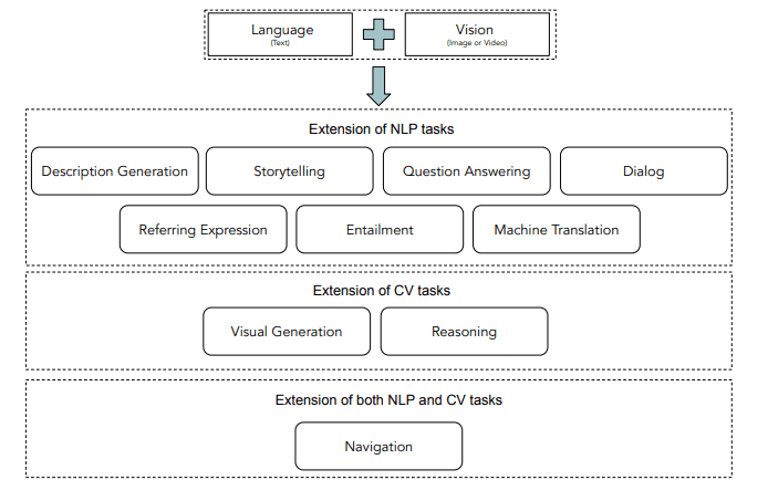
Taxonomy of popular visual language tasks
Depending on the task at hand, different architectures have been proposed over the years. In this article, we will explore some of the most popular ones.
BERT-like architectures
Given the incredible rise of transformers in NLP, it was inevitable that people would also try to apply them in VL tasks. The majority of papers have been used some version of BERT, resulting in a simultaneous explosion of BERT-like multimodal models: VisualBERT, ViLBERT, Pixel-BERT, ImageBERT, VL-BERT, VD-BERT, LXMERT, UNITER. They are all based on the same idea: they process language and images at the same time with a transformer-like architecture. We generally divide them into two categories: two-stream models and single-stream models.
Two-stream models: ViLBERT
Two-stream model is a literature term that refers to VL models which process text and images using two separate modules. ViLBERT and LXMERT fall into this category. ViLBERT is trained on image-text pairs. The text is encoded with the standard transformer process using tokenization and positional embeddings. It is then processed by the self-attention modules of the transformer. Images are decomposed into non-overlapping patches projected in a vector, as in vision transformer’s patch embeddings. To learn a joint representation of images and text, a “co-attention” module is used. The “co-attention” module calculates importance scores based on both images and text embeddings.
Source: OpenAI’s blog
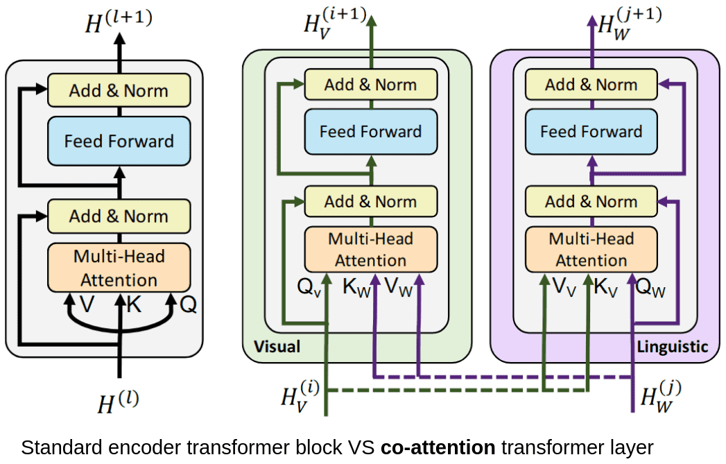
VilBERT processes images and text in two parallel streams that interact through co-attention
The two sides of the model are initialized separately. Regarding the text stream (purple), the weights are set by pretraining the model on a standard text corpus, while for the image stream (green), a Faster R-CNN is used. The entire model is trained on a dataset of image-text pairs with the end objective being to understand the relationship between text and images. The pretrained model can then be fine-tuned to a variety of downstream VL tasks.
Single-stream models
In contrast, models such as VisualBERT, VL-BERT, UNITER encode both modalities within the same module. For example, VisualBERT combines image regions and language with a transformer in order for self-attention to discover alignments between them. In essence, they added a visual embedding to the standard BERT architecture. The visual embedding consists of:
A visual feature representation of the region produced by a CNN
A segment embedding that distinguishes image from text embeddings
A positional embedding to align regions with words if provided in the input
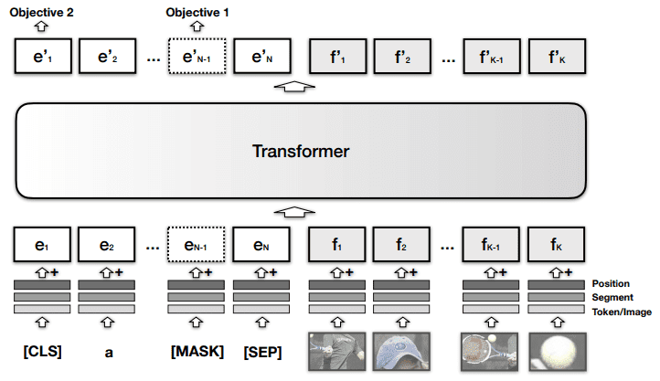
VisualBERT combines image regions and text with a transformer module
Pretraining and fine-tuning
The performance benefits of these models are partially due to the fact that they are pretrained on huge datasets. Visual BERT-like models are usually pretrained on paired image + text datasets, learning general multimodal representations. Afterwards, they are fine-tuned on downstream tasks such as visual question answering (VQA), etc with specific datasets.
Let’s explore some common pretraining strategies.
Pretraining strategies
Masked Language Modeling is often used when the transformer is trained only on text. Certain tokens of the input are being masked at random. The model is trained to simply predict the masked tokens (words). In the case of BERT, bidirectional training enables the model to use both previous and following tokens as context for prediction.
Next Sequence Prediction works again only with text as input and evaluates if a sentence is an appropriate continuation of the input sentence. By using both false and correct sentences as training data, the model is able to capture long-term dependencies.
Masked Region Modeling masks image regions in a similar way to masked language modeling. The model is then trained to predict the features of the masked region.
Image-Text Matching forces the model to predict if a sentence is appropriate for a specific image.
Word-Region Alignment finds correlations between image region and words.
Masked Region Classification predicts the object class for each masked region.
Masked Region Feature Regression learns to regress the masked image region to its visual features.
For example, VisualBERT is pretrained with the Masked Language Modeling and Image-text matching on an image-caption dataset.
The above methods create supervised learning objectives. Either the label is derived from the input, aka self-supervised or a labeled dataset (usually image-text pairs) is used. Are there any other attempts? Of course.
The following strategies are also used in VL modeling. They are often combined on various proposals.
Unsupervised VL Pretraining usually refers to pretraining without paired image-text data but rather with a single modality. During fine-tuning though, the model is fully-supervised.
Multi-task Learning is the concept of joint learning across multiple tasks in order to transfer the learnings from one task to another.
Contrastive Learning is used to learn visual-semantic embeddings in a self-supervised way. The main idea is to learn such an embedding space in which similar pairs stay close to each other while dissimilar ones are far apart.
Zero-shot learning is the ability to generalize at inference time on samples from unseen classes.
Let’s now proceed with some of the most popular architectures.
VL Generative models
DALL-E
DALL-E tackles the visual generation (VG) problem by being able to generate accurate images from a text description. The architecture is again trained with a text-images pair dataset.
DALL-E uses a discrete variational autoencoder (dVAE ) to map the images to image tokens. dVAE essentially uses a discrete latent space compared to a typical VAE. The text is tokenized with byte-pair encoding. The image and text tokens are concatenated and processed as a single data stream.
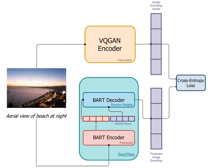
Training pipeline of DALL-E mini, slightly different from the original DALL-e
DALL-E uses an autoregressive transformer to process the stream in order to model the joint distribution of text and images. In the transformer’s decoder, each image can attend to all text tokens. At inference time, we concatenate the tokenized target caption with a sample from the dVAE, and pass the data stream to the autoregressive decoder, which will output a novel token image.
DALL-E provides some exceptional results (although admittedly a little cartoonized) as you can see in the image below.

DALL-E generates realistic images based on a textual description. Source: DALL·E: Creating Images from Text
GLIDE
Following the work of DALLE, GLIDE is another generative model that seems to outperform previous efforts. GLIDE is essentially a diffusion model.

Diffusion models consists of multiple diffusion steps that slowly add random noise to the data. Then, they aim to learn to reverse the diffusion process to construct samples from the data distribution from noise. Source: lilianweng
Diffusion models, in a nutshell, work by slowly injecting random noise to the data in a sequential fashion (formulated as a Markov chain). They then learn to reverse the process in order to construct novel data from the noise. So instead of sampling from the original unknown data distribution, they can sample from a known data distribution produced after a series of diffusion steps. In fact, it can be proved that if we add gaussian noise, the end (limit) distribution will be a typical normal distribution.
The diffusion model receives input as images and can output novel ones. But it can also be conditioned on textual information so that the generated image will be appropriate for specific text inputs. And that’s exactly what GLIDE does. It experiments with a variety of methods to “guide” the diffusion models.
Mathematically, the diffusion process can be formulated as follows. If we take a sample xixixi from a data distribution q(x0)q(x_0)q(x0), we can produce a Markov chain of latent variables x1,…xTx_1, … x_Tx1,…xT by progressively adding Gaussian noise of magnitude 1−at1-a_t1−at:
q(xt∣xt−1):=N(xt;atxt−1,(1−at)I) q(x_t | x_{t-1}) := N(x_t;\sqrt{a_t}x_{t-1}, (1-a_t)I) q(xt∣xt−1):=N(xt;atxt−1,(1−at)I)
That way, we can well-define the posterior q(xt−1∣xt)q_(x_{t-1}| x_t)q(xt−1∣xt) and approximate it using a model pθ(xt−1∣xt)p_{\theta}(x_{t-1}| x_t)pθ(