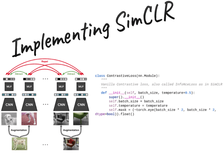
In this hands-on tutorial, we will provide you with a reimplementation of SimCLR self-supervised learning method for pretraining robust feature extractors. This method is fairly general and can be applied to any vision dataset, as well as different downstream tasks.
In a previous tutorial, I wrote a bit of a background on the self-supervised learning arena. Time to get into your first project by running SimCLR on a small dataset with 100K unlabelled images called STL10.
Code is available on Github.
The SimCLR method: contrastive learning
Let sim(u,v)sim(u,v)sim(u,v) note the dot product between 2 normalized uuu and vvv vectors (i.e. cosine similarity).
Then the loss function for a positive pair of examples (i,j) is defined as:
ℓi,j=−logexp(sim(zi,zj)/τ)∑k=12N1[k≠i]exp(sim(zi,zk)/τ)\ell_{i, j}=-\log \frac{\exp \left(\operatorname{sim}\left(\boldsymbol{z}_{i}, \boldsymbol{z}_{j}\right) / \tau\right)}{\sum_{k=1}^{2 N} \mathbb{1}_{[k \neq i]} \exp \left(\operatorname{sim}\left(\boldsymbol{z}_{i}, \boldsymbol{z}_{k}\right) / \tau\right)}ℓi,j=−log∑k=12N1[k=i]exp(sim(zi,zk)/τ)exp(sim(zi,zj)/τ)
where 1[k≠i]∈0,1\mathbb{1}_{[k \neq i]} \in {0,1}1[k=i]∈0,1 is an indicator function evaluating to 1 iff k!=ik != ik!=i. For more info on that check how we are going to index the similarity matrix to get the positives and the negatives.
τ\tauτ denotes a temperature parameter. The final loss is computed by summing all positive pairs and divide by 2×N=views×batch_size2\times N = views \times batch\_size2×N=views×batch_size
There are different ways to develop contrastive loss. Here we provide you with some important info.
L2 normalization and cosine similarity matrix calculation
First, one needs to apply an L2 normalization to the features, otherwise, this method does not work. L2 normalization means that the vectors are normalized such that they all lie on the surface of the unit (hyper)sphere, where the L2 norm is 1.
z_i = F.normalize(proj_1, p=2, dim=1)
z_j = F.normalize(proj_2, p=2, dim=1)
Concatenate the 2 output views in the batch dimension. Their shape will be [2×batch_size,dim][2 \times batch\_size, dim][2×batch_size,dim]. Then, calculate the similarity/logits of all pairs. This can be implemented by a matrix multiplication as follows. The output shape is equal to [batch_size×views,batch_size×views][batch\_size \times views, batch\_size \times views][batch_size×views,batch_size×views]
def calc_similarity_batch(self, a, b):
representations = torch.cat([a, b], dim=0)
return F.cosine_similarity(representations.unsqueeze(1), representations.unsqueeze(0), dim=2)
…
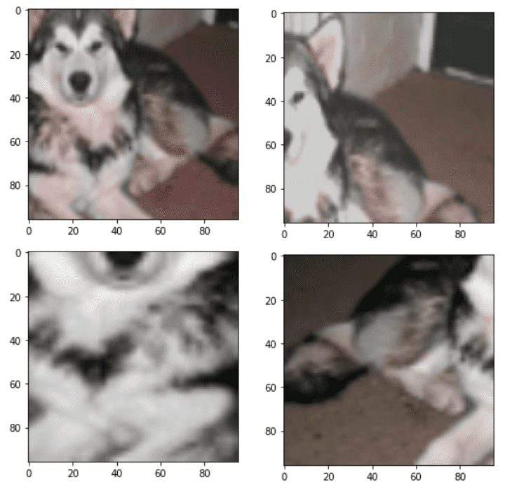
Below are 4 different views of the same image by applying the same stochastic pipeline:

To visualize them you need to undo the mean-std normalization and put the color channels in the last dimension:
def imshow(img):
“””
shows an imagenet-normalized image on the screen
“””
mean = torch.tensor([0.485, 0.456, 0.406], dtype=torch.float32)
std = torch.tensor([0.229, 0.224, 0.225], dtype=torch.float32)
unnormalize = T.Normalize((-mean / std).tolist(), (1.0 / std).tolist())
npimg = unnormalize(img).numpy()
plt.imshow(np.transpose(npimg, (1, 2, 0)))
plt.show()
dataset = STL10(“./”, split=’train’, transform=Augment(96), download=True)
imshow(dataset[99][0][0])
imshow(dataset[99][0][0])
imshow(dataset[99][0][0])
imshow(dataset[99][0][0])
To continue reading, please visit the website.