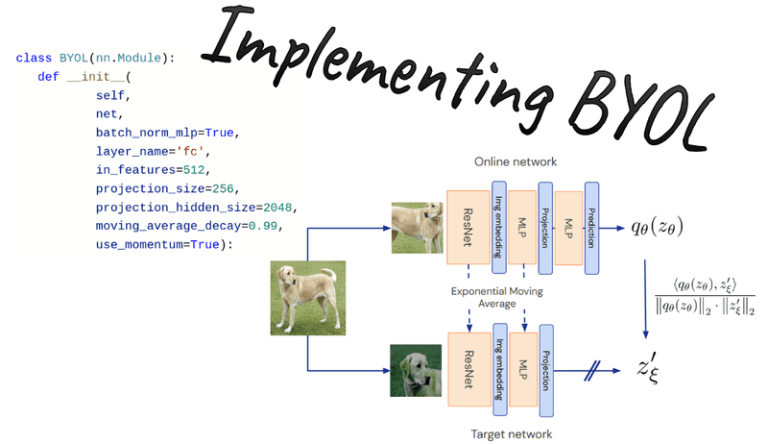
After presenting SimCLR, a contrastive self-supervised learning framework, I decided to demonstrate another infamous method, called BYOL. Bootstrap Your Own Latent (BYOL), is a new algorithm for self-supervised learning of image representations. BYOL has two main advantages:
It does not explicitly use negative samples. Instead, it directly minimizes the similarity of representations of the same image under a different augmented view (positive pair). Negative samples are images from the batch other than the positive pair.
As a result, BYOL is claimed to require smaller batch sizes, which makes it an attractive choice.
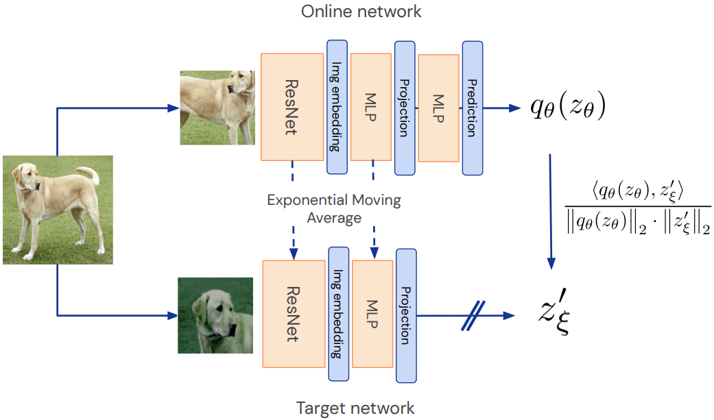
Below, you can examine the method. Unlike the original paper, I call the online network student and the target network teacher.

Overview of BYOL method. Source: BYOL paper
Online network aka student: compared to SimCLR, there is a second MLP, called predictor, which makes the whole method asymmetric. Asymmetric compared to what? Well, to the teacher model (target network).
Why is that important?
Because the teacher model is updated only through exponential moving average (EMA) from the student’s parameters. Ultimately, at each iteration, a tiny percentage (less than 1%) of the parameters of the student is passed to the teacher. Thus, gradients flow only through the student network. This can be implemented as:
class EMA():
def __init__(self, alpha):
super().__init__()
self.alpha = alpha
def update_average(self, old, new):
if old is None:
return new
return old * self.alpha + (1 – self.alpha) * new
ema = EMA(0.99)
for student_params, teacher_params in zip(student_model.parameters(),teacher_model.parameters()):
old_weight, up_weight = teacher_params.data, student_params.data
teacher_params.data = ema.update_average(old_weight, up_weight)
Another key difference between Simclr and BYOL is the loss function.
Loss function
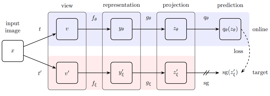
The predictor MLP is only applied to the student, making the architecture asymmetric. This is a key design choice to avoid mode collapse. Mode collapse here would be to output the same projection for all the inputs.

Overview of BYOL method. Source: BYOL paper
Finally, the authors defined the following mean squared error between the L2-normalized predictions and target projections:
The L2 loss can be implemented as follows. L2 normalization is applied beforehand.
import torch
import torch.nn.functional as F
def loss_fn(x, y):
x = F.normalize(x, dim=-1, p=2)
y = F.normalize(y, dim=-1, p=2)
return 2 – 2 * (x * y).sum(dim=-1)
Code is available on GitHub
Tracking down what’s happening in self-supervised pretraining: KNN accuracy
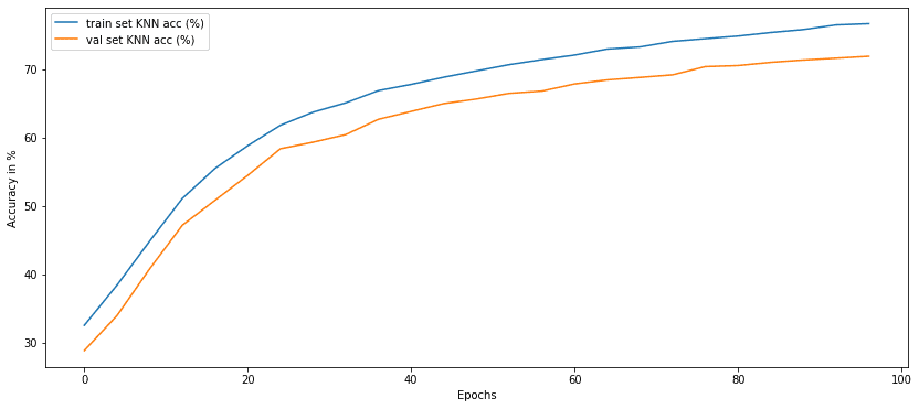
Nonetheless, the loss in self-supervised learning is not a reliable metric to track. What I found out to be the best way to track what’s happening while training, is to measure the ΚΝΝ accuracy.
The critical advantage of using KNN is that we don’t have to train a linear classifier on top each time, so it’s faster and completely unsupervised.
Note: Measuring KNN only applies to image classification, but you get the idea. For this purpose, I made a class to encapsulate the logic of KNN in our context:
import numpy as np
import torch
from sklearn.model_selection import cross_val_score
from sklearn.neighbors import KNeighborsClassifier
from torch import nn
class KNN():
def __init__(self, model, k, device):
super(KNN, self).__init__() self.k = k
self.device = device
self.model = model.to(device)
self.model.eval()
def extract_features(self, loader):
“””
Infer/Extract features from a trained model
Args:
loader: train or test loader
Returns: 3 tensors of all: input_images, features, labels
“””
x_lst = []
features = []
label_lst = []
with torch.no_grad():
for input_tensor, label in loader:
h = self.model(input_tensor.to(self.device))
features.append(h)
x_lst.append(input_tensor)
label_lst.append(label)
x_total = torch.stack(x_lst)
h_total = torch.stack(features)
label_total = torch.stack(label_lst)
return x_total, h_total, label_total
def knn(self, features, labels, k=1):
“””
Evaluating knn accuracy in feature space.
Calculates only top-1 accuracy (returns 0 for top-5)
Args:
features: [… , dataset_size, feat_dim]
labels: [… , dataset_size]
k: nearest neighbours
Returns: train accuracy, or train and test acc
“””
feature_dim = features.shape[-1]
with torch.no_grad():
features_np = features.cpu().view(-1, feature_dim).numpy()
labels_np = labels.cpu().view(-1).numpy()
self.cls = KNeighborsClassifier(k, metric=”cosine”).fit(features_np, labels_np)
acc = self.eval(features, labels)
return acc
def eval(self, features, labels):
feature_dim = features.shape[-1]
features = features.cpu().view(-1, feature_dim).numpy()
labels = labels.cpu().view(-1).numpy()
acc = 100 * np.mean(cross_val_score(self.cls, features, labels))
return acc
def _find_best_indices(self, h_query, h_ref):
h_query = h_query / h_query.norm(dim=1).view(-1, 1)
h_ref = h_ref / h_ref.norm(dim=1).view(-1, 1)
scores = torch.matmul(h_query, h_ref.t())
score, indices = scores.topk(1, dim=1)
return score, indices
def fit(self, train_loader, test_loader=None):
with torch.no_grad():
x_train, h_train, l_train = self.extract_features(train_loader)
train_acc = self.knn(h_train, l_train, k=self.k)
if test_loader is not None:
x_test, h_test, l_test = self.extract_features(test_loader)
test_acc = self.eval(h_test, l_test)
return train_acc, test_acc
Now we can focus on the method and BYOL model.
Modify resnet: add MLP projection heads
We will start with a base model (resnet18) and modify it for self-supervised learning. The last layer that normally does the classification is replaced with an identity function. The output features of resnet18 will be fed to the MLP projector.
import copy
import torch
from torch import nn
import torch.nn.functional as F
class MLP(nn.Module)
def __init__(self, dim, embedding_size=256, hidden_size=2048, batch_norm_mlp=False):
super().__init__()
norm = nn.BatchNorm1d(hidden_size) if batch_norm_mlp else nn.Identity()
self.net = nn.Sequential(
nn.Linear(dim, hidden_size),
norm,
nn.ReLU(inplace=True),
nn.Linear(hidden_size, embedding_size)
)
def forward(self, x):
return self.net(x)
class AddProjHead(nn.Module):
def __init__(self, model, in_features, layer_name, hidden_size=4096,
embedding_size=256, batch_norm_mlp=True):
super(AddProjHead, self).__init__()
self.backbone = model
setattr(self.backbone, layer_name, nn.Identity())
self.backbone.conv1 = torch.nn.Conv2d(3, 64, kernel_size=3, stride=1, padding=1, bias=False)
self.backbone.maxpool = torch.nn.Identity()
self.projection = MLP(in_features, embedding_size, hidden_size=hidden_size, batch_norm_mlp=batch_norm_mlp)
def forward(self, x, return_embedding=False):
embedding = self.backbone(x)
if return_embedding:
return embedding
return self.projection(embedding)
I also replaced the first conv layer of resnet18 from 7×7 to 3×3 convolution since we are playing with 32×32 images (CIFAR-10).
Code is available on GitHub. If you are planning to solidify your Pytorch knowledge, there are two amazing books that we highly recommend: Deep learning with PyTorch from Manning Publications and Machine Learning with PyTorch and Scikit-Learn by Sebastian Raschka. You can always use the 35% discount code blaisummer21 for all Manning’s products.
The actual BYOL method

Deep Learning in Production Book 📖
Learn how to build, train, deploy, scale and maintain deep learning models. Understand ML infrastructure and MLOps using hands-on examples. Learn more
* Disclosure: Please note that some of the links above might be affiliate links, and at no additional cost to you, we will earn a commission if you decide to make a purchase after clicking through.