A U-shaped architecture consists of a specific encoder-decoder scheme: The encoder reduces the spatial dimensions in every layer and increases the channels. On the other hand, the decoder increases the spatial dims while reducing the channels. The tensor that is passed in the decoder is usually called bottleneck. In the end, the spatial dims are restored to make a prediction for each pixel in the input image. These kinds of models are extremely utilized in real-world applications.
This article aims to explore the Unet architectures that stood the test of time.
To dive deeper into how AI is used in Medicine, you can’t go wrong with this online course by Coursera: AI for Medicine
Fully Convolutional Network (FCN)
Fully convolutional network 1 was one of the first architectures without fully connected layers. Apart from the fact that it can be trained end-to-end, for individual pixel prediction (e.g semantic segmentation), it can process arbitrary-sized inputs. It is a general architecture that effectively uses transposed convolutions as a trainable upsampling method.
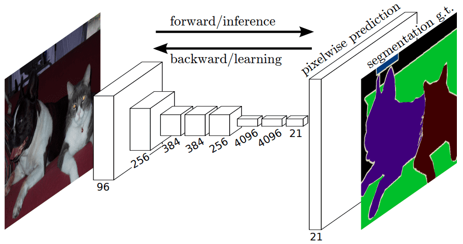
The fully convolutional layer architecture. Source
Given a pretrained encoder here is what an FCN looks like:
import torch
import torch.nn as nn
class FCN32s(nn.Module):
def __init__(self, pretrained_net, n_class):
super().__init__()
self.n_class = n_class
self.pretrained_net = pretrained_net
self.relu = nn.ReLU(inplace=True)
self.deconv1 = nn.ConvTranspose2d(512, 512, kernel_size=3, stride=2, padding=1, dilation=1, output_padding=1)
self.bn1 = nn.BatchNorm2d(512)
self.deconv2 = nn.ConvTranspose2d(512, 256, kernel_size=3, stride=2, padding=1, dilation=1, output_padding=1)
self.bn2 = nn.BatchNorm2d(256)
self.deconv3 = nn.ConvTranspose2d(256, 128, kernel_size=3, stride=2, padding=1, dilation=1, output_padding=1)
self.bn3 = nn.BatchNorm2d(128)
self.deconv4 = nn.ConvTranspose2d(128, 64, kernel_size=3, stride=2, padding=1, dilation=1, output_padding=1)
self.bn4 = nn.BatchNorm2d(64)
self.deconv5 = nn.ConvTranspose2d(64, 32, kernel_size=3, stride=2, padding=1, dilation=1, output_padding=1)
self.bn5 = nn.BatchNorm2d(32)
self.classifier = nn.Conv2d(32, n_class, kernel_size=1)
def forward(self, x):
output = self.pretrained_net(x)
x5 = output[‘x5’]
score = self.bn1(self.relu(self.deconv1(x5)))
score = self.bn2(self.relu(self.deconv2(score)))
score = self.bn3(self.relu(self.deconv3(score)))
score = self.bn4(self.relu(self.deconv4(score)))
score = self.bn5(self.relu(self.deconv5(score)))
score = self.classifier(score)
return score
You can even load a pretrained model from pytorch hub:
import torch
model = torch.hub.load(‘pytorch/vision:v0.9.0’, ‘fcn_resnet101’, pretrained=True)
model.eval()
Note that all pre-trained models expect input images normalized in the same way, i.e. mini-batches of 3-channel RGB images of shape (N, 3, H, W), where N is the number of images, H and W are expected to be at least 224 pixels. The images have to be loaded in to a range of [0, 1] and then normalized using mean = [0.485, 0.456, 0.406] and std = [0.229, 0.224, 0.225]
U-Net and 3D U-Net
Later on, Unet modifies and extends FCN.
The main idea is to make FCN maintain the high-level features in the early layer of the decoder. To this end, they introduce long skip-connections to localize the segmentations.
In this manner, high-resolution features (but semantically low) from the encoder path are combined and reused with the upsampled output. Unet is also a symmetric architecture, as depicted below.
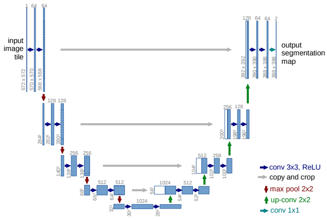
The Unet model. Source
It can be divided into an encoder-decoder path or contracting-expansive path equivalently.
Encoder (left side): It consists of the repeated application of two 3×3 convolutions. Each conv is followed by a ReLU and batch normalization. Then a 2×2 max pooling operation is applied to reduce the spatial dimensions. Again, at each downsampling step, we double the number of feature channels, while we cut in half the spatial dimensions.
Decoder path (right side): Every step in the expansive path consists of an upsampling of the feature map followed by a 2×2 transpose convolution, which halves the number of feature channels. We also have a concatenation with the corresponding feature map from the contracting path, and usually a 3×3 convolutional (each followed by a ReLU). At the final layer, a 1×1 convolution is used to map the channels to the desired number of classes.
Here is an implementation of 2D Unet
import torch
import torch.nn as nn
import torch.nn.functional as F
class DoubleConv(nn.Module):
def __init__(self, in_ch, out_ch):
super(DoubleConv, self).__init__()
self.conv = nn.Sequential(
nn.Conv2d(in_ch, out_ch, 3, padding=1),
nn.BatchNorm2d(out_ch),
nn.ReLU(inplace=True),
nn.Conv2d(out_ch, out_ch, 3, padding=1),
nn.BatchNorm2d(out_ch),
nn.ReLU(inplace=True))
def forward(self, x):
x = self.conv(x)
return x
class InConv(nn.Module):
def __init__(self, in_ch, out_ch):
super(InConv, self).__init__()
self.conv = DoubleConv(in_ch, out_ch)
def forward(self, x):
x = self.conv(x)
return x
class Down(nn.Module):
def __init__(self, in_ch, out_ch):
super(Down, self).__init__()
self.mpconv = nn.Sequential(
nn.MaxPool2d(2),
DoubleConv(in_ch, out_ch)
)
def forward(self, x):
x = self.mpconv(x)
return x
class Up(nn.Module):
def __init__(self, in_ch, out_ch, bilinear=True):
super(Up, self).__init__()
if bilinear:
self.up = nn.Upsample(scale_factor=2, mode=’bilinear’, align_corners=True)
else:
self.up = nn.ConvTranspose2d(in_ch // 2, in_ch // 2, 2, stride=2)
self.conv = DoubleConv(in_ch, out_ch)
def forward(self, x1, x2):
x1 = self.up(x1)
diffY = x2.size()[2] – x1.size()[2]
diffX = x2.size()[3] – x1.size()[3]
x1 = F.pad(x1, (diffX // 2, diffX – diffX // 2,
diffY // 2, diffY – diffY // 2))
x = torch.cat([x2, x1], dim=1)
x = self.conv(x)
return x
class OutConv(nn.Module):
def __init__(self, in_ch, out_ch):
super(OutConv, self).__init__()
self.conv = nn.Conv2d(in_ch, out_ch, 1)
def forward(self, x):
x = self.conv(x)
return x
class Unet(nn.Module):
def __init__(self, in_channels, classes):
super(Unet, self).__init__()
self.n_channels = in_channels
self.n_classes = classes
self.inc = InConv(in_channels, 64)
self.down1 = Down(64, 128)
self.down2 = Down(128, 256)
self.down3 = Down(256, 512)
self.down4 = Down(512, 512)
self.up1 = Up(1024, 256)
self.up2 = Up(512, 128)
self.up3 = Up(256, 64)
self.up4 = Up(128, 64)
self.outc = OutConv(64, classes)
def forward(self, x):
x1 = self.inc(x)
x2 = self.down1(x1)
x3 = self.down2(x2)
x4 = self.down3(x3)
x5 = self.down4(x4)
x = self.up1(x5, x4)
x = self.up2(x, x3)
x = self.up3(x, x2)
x = self.up4(x, x1)
x = self.outc(x)
return x
This method has great success in 2D biomedical image segmentation. And it is still used as a baseline method. But what about 3D images?
The 3D-Unet
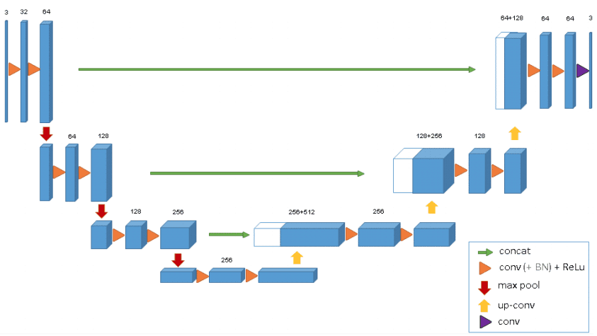
3D Unet was introduced shortly after Unet to process volumes. Only 3 layers are shown in the official diagram but in practice, we use more when we implement this model. Each block uses batch normalization after the convolution.
V-Net (2016)
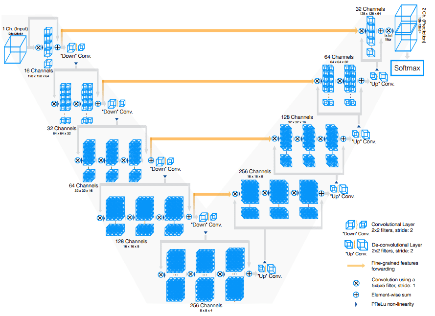
Vnet extends Unet to process 3D MRI volumes. In contrast to processing the input 3D volumes slice-wise, they proposed to use 3D convolutions. In the end, medical images have an inherent 3D structure, and slice-wise processing is sub-optimal. The main modifications of Vnet are:
Motivated by similar works on image classification, they replaced max-pooling operations with strided convolutions. This is performed through convolution with 2 × 2 × 2 kernels applied with stride 2.
3D convolutions with padding are performed in each stage using 5×5×5 kernels.
Short residual connections are also employed in both parts of the network.
They use 3D transpose convolutions in order to increase the size of the inputs, followed by one to three conv layers. Feature maps are halved in every decoder layer.
All the above can be illustrated in this image:
UNet++ (2018)
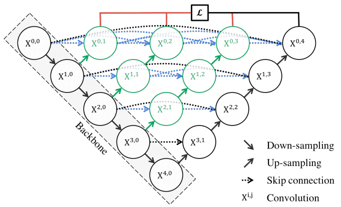
Motivation: The skip connections used in U-Net directly fast-forward high-resolution feature maps from the encoder to the decoder network. This results in the concatenation of semantically dissimilar feature maps.
The main idea behind UNet++ is to bridge the semantic gap between the feature maps of the encoder and decoder before concatenation. To this end, UNet++ is based on both nested and dense skip connections. UNet++ can effectively capture fine-grained details of 2D images. Visually:
